# DeepLearning_PlantDiseases
**Repository Path**: heyihuiforjava/DeepLearning_PlantDiseases
## Basic Information
- **Project Name**: DeepLearning_PlantDiseases
- **Description**: Training and evaluating state-of-the-art deep learning CNN architectures for plant disease classification task.
- **Primary Language**: Unknown
- **License**: Not specified
- **Default Branch**: master
- **Homepage**: None
- **GVP Project**: No
## Statistics
- **Stars**: 0
- **Forks**: 0
- **Created**: 2020-05-29
- **Last Updated**: 2025-11-18
## Categories & Tags
**Categories**: Uncategorized
**Tags**: None
## README
# Deep Learning for the plant disease detection
This is the source code of the experiment described in chapter [Deep Learning for Plant Diseases: Detection and Saliency Map Visualisation](https://link.springer.com/chapter/10.1007/978-3-319-90403-0_6) in a book **Human and Machine Learning, 2018**.
Training and evaluating state-of-the-art deep architectures for plant disease classification task using pyTorch.
Models are trained on the preprocessed dataset which can be downloaded [here](https://drive.google.com/open?id=0B_voCy5O5sXMTFByemhpZllYREU).
Dataset is consisted of **38** disease classes from [PlantVillage](https://plantvillage.org/) dataset and **1** background class from Stanford's open dataset of background images - [DAGS](http://dags.stanford.edu/projects/scenedataset.html).
**80%** of the dataset is used for training and **20%** for validation.
## Usage:
1. Train all the models with **train.py** and store the evaluation stats in **stats.csv**:
`python3 train.py`
2. Plot the models' results for every archetecture based on the stored stats with **plot.py**:
`python3 plot.py`
## Results:
The models on the graph were retrained on final fully connected layers only - **shallow**, for the entire set of parameters - **deep** or from its initialized state - **from scratch**.
| Model | Training type |Training time [~h] | Accuracy Top 1|
| ------------- |:-------------:|:-----------------:|:-------------:|
| AlexNet | shallow | 0.87 | 0.9415 |
| AlexNet | from scratch | 1.05 | 0.9578 |
| AlexNet | deep | 1.05 | 0.9924 |
| **DenseNet169** | **shallow** | **1.57** | **0.9653** |
| **DenseNet169** | **from scratch** | **3.16** | **0.9886** |
| DenseNet169 | deep | 3.16 | 0.9972 |
| Inception_v3 | shallow | 3.63 | 0.9153 |
| Inception_v3 | from scratch | 5.91 | 0.9743 |
| **Inception_v3**| **deep** | **5.64** | **0.9976** |
| ResNet34 | shallow | 1.13 | 0.9475 |
| ResNet34 | from scratch | 1.88 | 0.9848 |
| ResNet34 | deep | 1.88 | 0.9967 |
| Squeezenet1_1 | shallow | 0.85 | 0.9626 |
| Squeezenet1_1 | from scratch | 1.05 | 0.9249 |
| Squeezenet1_1 | deep | 2.10 | 0.992 |
| VGG13 | shallow | 1.49 | 0.9223 |
| VGG13 | from scratch | 3.55 | 0.9795 |
| VGG13 | deep | 3.55 | 0.9949 |
**NOTE**: All the others results are stored in [stats.csv](https://github.com/MarkoArsenovic/DeepLearning_PlantDiseases/blob/master/Results/stats.csv)
## Graph

## Visualization Experiments
**@Contributor**: [Brahimi Mohamed](mailto:m_brahimi@esi.dz)
## Prerequisites:
Train the new model or download pretrained models on **10 classes** of **Tomato** from PlantVillage dataset: [AlexNet](https://drive.google.com/open?id=1Ms1Ri5DUy_D4uYZX5tG2hrN2hUH6XbQS) or [VGG13](https://drive.google.com/open?id=1f0nPNRfL42fJA8tF5JoKUKv0Xr98p8-P).
## Occlusion Experiment
Occlusion experiments for producing the heat maps that show visually the influence of each region on the classification.
### Usage:
Produce the heat map and plot with **occlusion.py** and store the visualizations in **output_dir**:
`python3 occlusion.py /path/to/dataset /path/to/output_dir model_name.pkl /path/to/image disease_name`
### Visualization Examples on AlexNet:
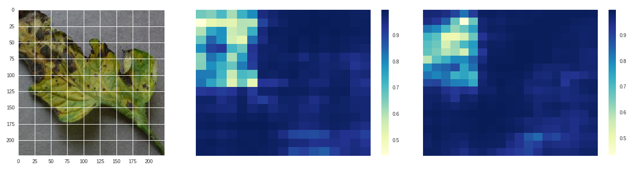
*Early blight - original, size 80 stride 10, size 100 stride 10*
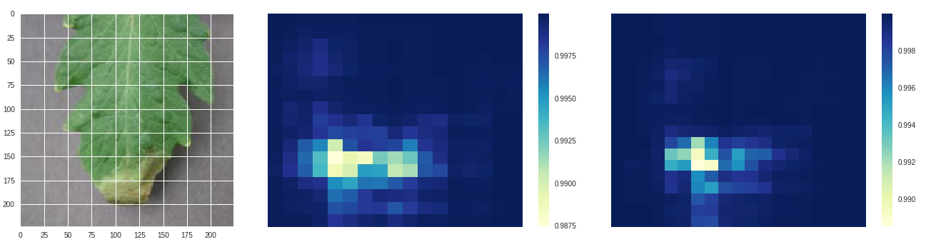
*Late blight - original, size 80 stride 10, size 100 stride 10*
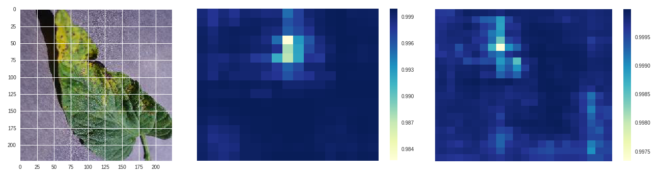
*Septoria leaf spot - original, size 50 stride 10, size 100 stride 10*
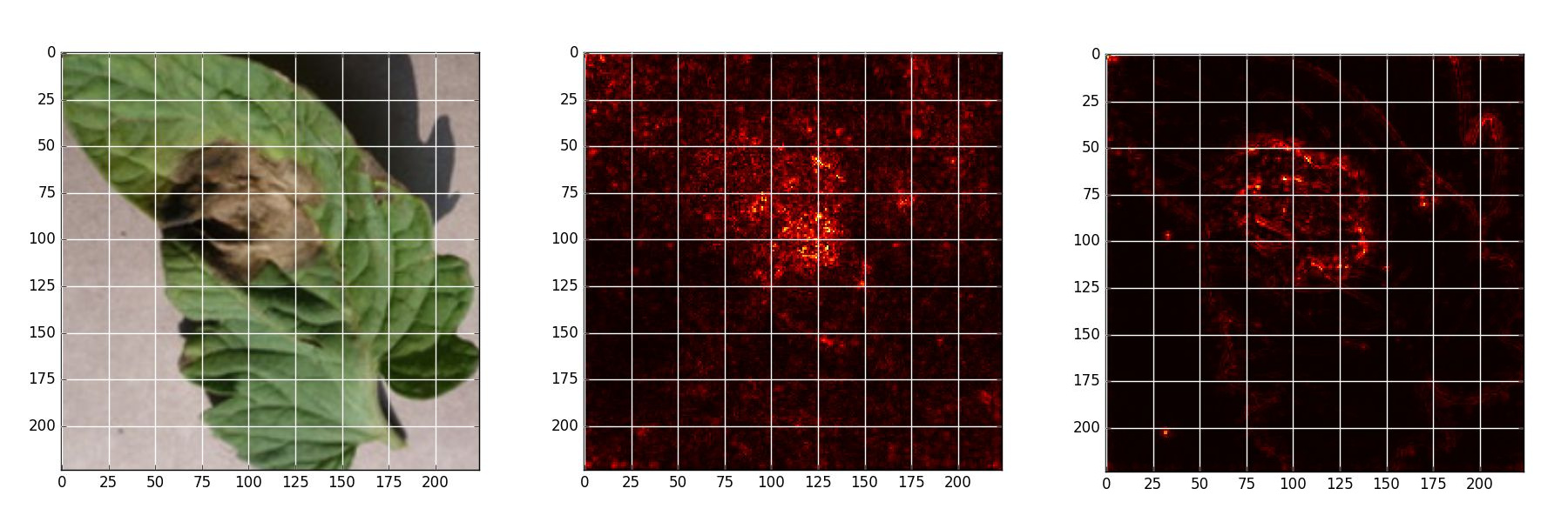
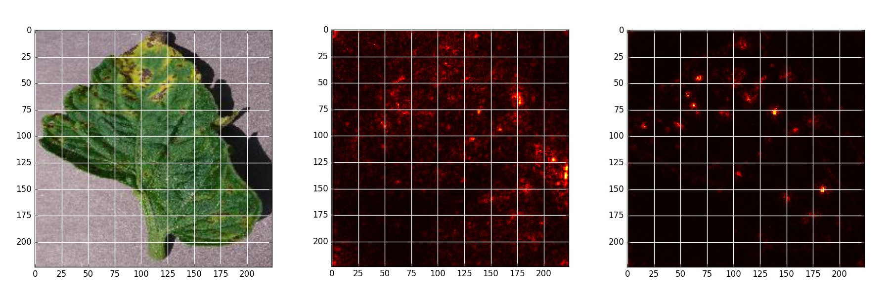
## Saliency Map Experiment
Saliency map is an analytical method that allows to estimate theimportance of each pixel, using only one forward and one backward pass through the network.
### Usage:
Produce the visualization and plot with **saliency.py** and store the visualizations in **output_dir**:
`python3 occlusion.py /path/to/model /path/to/dataset /path/to/image class_name`
### Visualization Examples on VGG13:
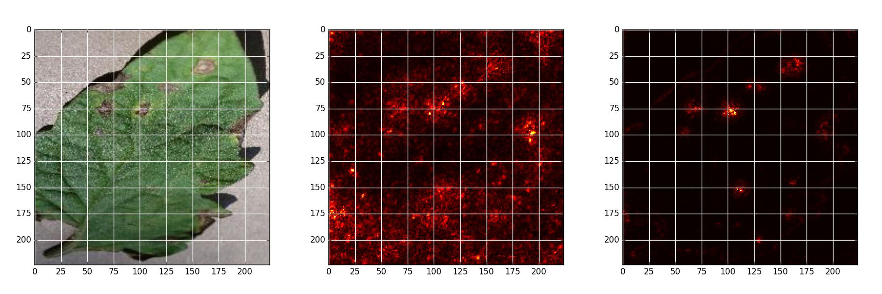
*Early blight - Original, Naive backpropagation , Guided backpropagation*
*Late blight - Original, Naive backpropagation , Guided backpropagation*
*Septoria leaf spot - Original, Naive backpropagation , Guided backpropagation*
---
NOTE: When using (any part) of this repository, please cite [Deep Learning for Plant Diseases: Detection and Saliency Map Visualisation](https://link.springer.com/chapter/10.1007/978-3-319-90403-0_6):
```
@Inbook{Brahimi2018,
author = "Brahimi, Mohammed and Arsenovic, Marko and Laraba, Sohaib and Sladojevic, Srdjan and Boukhalfa, Kamel and Moussaoui, Abdelouhab",
editor = "Zhou, Jianlong and Chen, Fang",
title = "Deep Learning for Plant Diseases: Detection and Saliency Map Visualisation",
bookTitle = "Human and Machine Learning: Visible, Explainable, Trustworthy and Transparent", year="2018",
publisher = "Springer International Publishing",
address = "Cham",
pages = "93--117",
url = "https://doi.org/10.1007/978-3-319-90403-0_6"
}
```